Part 2
Measures of Spread and Center
| Measure | Female Household Headed Families | Male Household Headed Families |
|---|---|---|
| Mean | 22378.82 | 6580.667 |
| Median | 6654 | 2467 |
| Variance | 1304129049 | 110608654 |
| Standard Deviation | 36112.73 | 10517.06 |
The mean and median are different in both cases. This is not surprising since as seen from the previous graphs, the female’s household image has a greater range in the x-axis compared to the male’s one. Furthermore when looking at the graph distributions, both are skewed to the right, but the tot female household graph has greater mean compared to the male’s; this might be attributed to the disparity in income, which would explain the great difference in numbers. Additionally, the Total Male Household Headed Families has a standard deviation that is fairly close to the mean, again showing that the graph a smaller spread across the data set
Scatterplots and Correlation
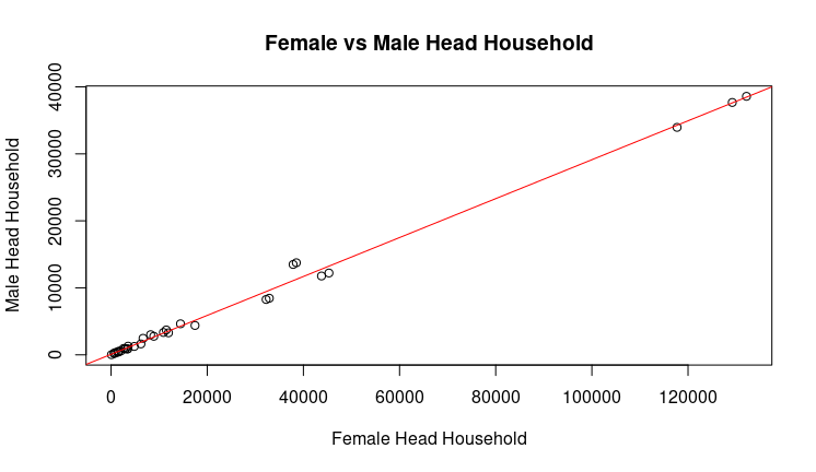
From the graph we can see that there appears to be a linear association between the Total Female Headed Household Families and Total Male Headed Household Families. The strong correlation of 0.9973634 between the two variables can be attributed by the need of families to rent a house or apartment, which causes the number of applicants to increase. Thus, the NYCHA will have a greater number of applicants. Additionally, there is a gap in the x-axis starting from 6000 to 8000, that is the same gap that was previously discussed, which might be caused by the lack of data for a period of time or the data might have been so small that they decided to ignore those values.
Confidence Interval
| Measure | Female Household Headed Families | Male Household Headed Families |
|---|---|---|
| Mean | 22378.82 | 6580.667 |
| Median | 6654 | 2467 |
| Variance | 1304129049 | 110608654 |
| Standard Deviation | 36112.73 | 10517.06 |
| Confidence Interval | [ 22189.65, 22567.99 ] | [ 6477.597, 6683.737 ] |
In both cases the confidence interval is positive, which is not surprising since the standard deviations have positive values. Moreover the mean falls within the interval range, suggesting that we can be 95% certain that we obtain the true mean. Another observation is the difference in values of the intervals from both data sets, which is caused by the distribution of the data being more spread in the female’s household graph compared to the male’s one.
Linear Regression
Equation of the Regression Line: y= 0.2905x + 80.4947. Where x is Total Female Headed Families and we are trying to predict the ratio between female to male household head:
The graph on the left is the same one as the previous when we looked at the correlation in the scatterplot. On the right we have the residual, which shows a normally distributed shape, suggesting the line is a good fit. This is confirmed by the R-Squared value of 0.99868, which indicates a strong linear association between the variables. Image of Scatter Plot with x-axis and residual y-axis The actual observed response value (x axis) vs. residual (y axis) graph illustrate that the residuals do not move/increase as the observed response value
Hypothesis
Test 1
Based on the NYCHA data, suppose we want to know if the percentage of females in charge of the family is higher than the male’s one. Upon taking a subset of the Total Male Headed Household Families and Total Female Headed Household Families, we found the mean to be 1626.792 and 5366.042, and sample sizes: 14438 and 19068 respectively. Can we conclude that there are more females in charge of families than males? Assuming that the significance level is 0.05:
Let μx be the mean of the Total Female Headed Household Families Let μy be the mean of the Total Male Headed Household Families
Null and Alternative Hypothesis: H0: μx = μx H1: μy > μy Test Statistic = 0.01598 Since the significance level is 0.05, the resulting = 0.05, with a critical value is zα = z0.05 = −1.64. With this information we reject the null hypothesis and conclude that there are more females in charge in the NYCHA programs that are in charge of the house.
Test 2
Based on the NYCHA data, suppose we want to know if the percentage of females in charge of the family is not the male’s one. Upon taking a subset of the Total Male Headed Household Families and Total Female Headed Household Families, we found the mean to be 342.375 and 469.6667, and sample sizes: 187 and 656 respectively. Can we conclude that there are more females in charge of families than males? Assuming that the significance level is 0.05
Let μx be the mean of the Total Female Headed Household Families Let μy be the mean of the Total Male Headed Household Families
Null and Alternative Hypothesis: H0: μx = μx H1: μy != μy Test Statistic = 0.01896 Since the significance level is 0.05, the resulting = 0.05, with a critical value is zα = z0.05 = −1.64. With this we can reject the null hypothesis since the test static is not in the critical value range. Thus conclude that the percentage of female to male in charge of the house based NYCHA is not the same.
Code Available on github